Moving to Euclidean space#

Before doing anything with the path integral, we Wick-rotate to Euclidean space. This means sending $x^0 = t \to -i\tau$, which turns the oscillatory $e^{iS}$ into a damped $e^{-S_E}$ — much better behaved for path integral manipulations.

The gauge field rotates too. Since $A_0$ sits in the same slot as $x^0$, it picks up a factor of $i$:

$A_0 \to iA_0^E$

while the spatial components $A_i$ are unchanged. This means the Minkowski contraction $A_\mu A^\mu = A_0^2 - A_i^2$ becomes $-(A_0^E)^2 - A_i^2 = -A_\mu^E A_\mu^E$ in Euclidean space. The relative sign between time and space components disappears — Euclidean space has no distinction between “upper” and “lower” indices, and everything just contracts with $\delta_{\mu\nu}$.

The field strength transforms similarly. Take $F_{0i} = \partial_0 A_i - \partial_i A_0$. After the rotation, each time derivative $\partial_0$ picks up an $i$, and $A_0 \to iA_0^E$, giving $F_{0i} \to iF_{0i}^E$. The Euclidean action for a massless $U(1)$ gauge field becomes:

$S_E[A] = \frac{1}{4}\int d^4x \; F_{\mu\nu}^E F_{\mu\nu}^E$

From here on, we’ll drop the $E$ superscripts — everything is Euclidean until further notice.

The operator you can’t invert#

Now let’s massage the action into a form that reveals the problem. The Lagrangian density is:

$\mathcal{L} = \frac{1}{4}F_{\mu\nu}F_{\mu\nu} = \frac{1}{4}(F_{0i}^2 + F_{ij}^2)$

We can write $F_{\mu\nu} = \partial_\mu A_\nu - \partial_\nu A_\mu$ and expand. After integrating by parts (throwing away boundary terms), the action takes the form:

$S[A] = \frac{1}{2}\int d^4x \; A_\mu\!\left(\Box\,\delta_{\mu\nu} - \partial_\mu\partial_\nu\right)A_\nu$

This is a quadratic action in $A_\mu$, which means the path integral is Gaussian. For a Gaussian integral to make sense, you need to invert the operator in the exponent — that inverse is the propagator. But the operator

$\mathcal{O}_{\mu\nu} = \Box\,\delta_{\mu\nu} - \partial_\mu\partial_\nu$

has a zero mode. To see this, hit it with $\partial_\mu\chi$ for any function $\chi$:

$\mathcal{O}_{\mu\nu}\,\partial_\nu\chi = \Box\,\partial_\mu\chi - \partial_\mu\partial_\nu\partial_\nu\chi = \Box\,\partial_\mu\chi - \partial_\mu\Box\chi = 0$

The operator annihilates any pure gauge configuration $\partial_\mu\chi$. A linear operator with zero modes has no inverse. No inverse means no propagator, and no propagator means the path integral

$Z = \int \mathcal{D}A_\mu \; e^{-S[A]}$

is not well-defined. We’re stuck.

But why does this zero mode exist? It’s not an accident — it’s a direct consequence of gauge invariance. The action doesn’t change under $A_\mu \to A_\mu + \partial_\mu\chi$, so the operator encoding the action must kill the pure-gauge directions. The kernel of $\mathcal{O}_{\mu\nu}$ is precisely the space of gauge transformations. This is the mathematical statement of the overcounting problem.

Two types of field configurations#

Let’s think about what the path integral $\int \mathcal{D}A_\mu$ is actually summing over. Every field configuration $A_\mu(x)$ contributes to this integral. But there are really two types of contributions:

1. Physically inequivalent configurations — these are the ones we want. They represent genuinely different states of the electromagnetic field, and summing over them gives the quantum behavior of the theory.

2. Gauge copies — for each physical configuration $A_\mu$, there is an entire family $\{A_\mu + \partial_\mu\chi\}$ of configurations related by gauge transformations. These all describe the same physics but the path integral counts each one separately.

The second type is the problem. We don’t just have one extra copy — we have one for every possible function $\chi(x)$, which is an infinite-dimensional family. The path integral includes a factor equal to the “volume” of this gauge orbit, and this volume is what makes the integral diverge.

What we’d like to do is split the measure:

$\int \mathcal{D}A_\mu = \int \mathcal{D}A_\text{phys} \times \int \mathcal{D}A_\text{gauge}$

and just throw away the gauge part. The challenge is doing this correctly.

Gauge orbits: the geometric picture#

The cleanest way to think about this is geometrical. Consider the (infinite-dimensional) space of all gauge field configurations $A_\mu(x)$.

Pick a particular configuration $A_\mu$. Now act on it with every possible gauge transformation:

$A_\mu^\chi = A_\mu + \partial_\mu\chi$

The set of all such $A_\mu^\chi$ as $\chi$ varies is called the gauge orbit of $A_\mu$, denoted $\mathcal{O}(A)$. Every point on this orbit is physically equivalent to $A_\mu$.

Now pick a different, physically inequivalent configuration $A_\mu'$ — meaning there is no gauge transformation taking $A_\mu$ to $A_\mu'$. It has its own orbit $\mathcal{O}(A')$, which doesn’t intersect $\mathcal{O}(A)$.

The full field space is foliated into these non-intersecting orbits. Physics lives on the space of orbits, not on individual configurations.

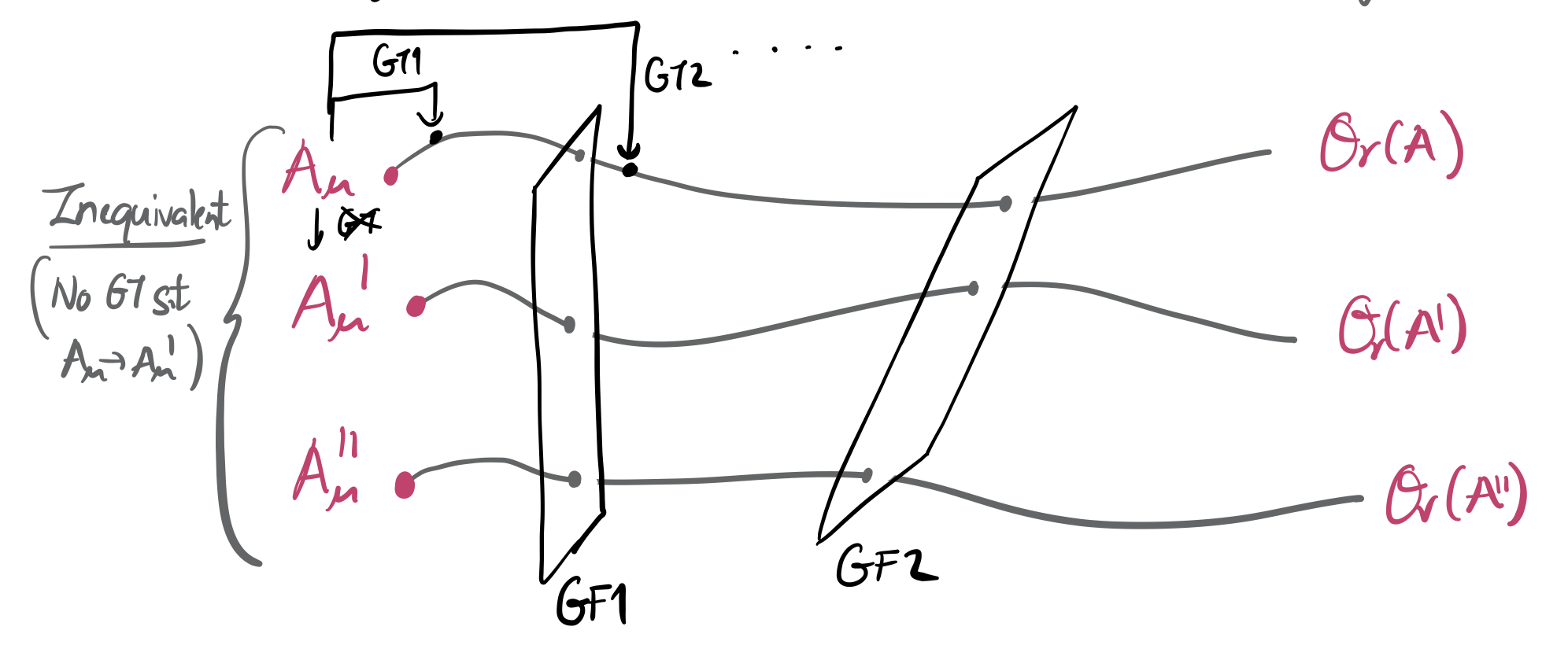
The horizontal curves are gauge orbits — each one represents a family of gauge-equivalent configurations. The pink dots ($A_\mu$, $A_\mu'$, $A_\mu''$) are physically inequivalent starting points, and the gauge transformations $GT_1, GT_2, \ldots$ slide you along an orbit without changing the physics. The vertical surfaces $GF_1, GF_2$ are gauge-fixing conditions — they slice through the orbits, picking out one representative from each.

A good gauge-fixing surface intersects each orbit exactly once. This is what we need: one configuration per orbit, no overcounting, no missing configurations. For $U(1)$ gauge theory in the perturbative regime, we can assume such a unique intersection exists. (For non-abelian theories, this assumption fails — a problem known as Gribov copies, which we’ll address in the non-abelian series.)

The Lorenz condition as a gauge-fixing surface#

The most common choice of gauge-fixing surface is the Lorenz condition:

$\partial_\mu A_\mu = 0$

Why does this pick one point per orbit? Start with any configuration $A_\mu$ and ask: can I find a $\chi$ such that the transformed field satisfies the condition?

$\partial_\mu A_\mu^\chi = \partial_\mu A_\mu + \Box\chi = 0$

This requires:

$\Box\chi = -\partial_\mu A_\mu$

which is just Poisson’s equation for $\chi$. With appropriate boundary conditions, it has a unique solution. So for every orbit, there is exactly one configuration satisfying $\partial_\mu A_\mu = 0$ — the Lorenz condition is a good gauge-fixing surface.

More generally, we can impose

$\partial_\mu A_\mu = G(x)$

for any fixed function $G(x)$. The required gauge transformation is then $\Box\chi = G(x) - \partial_\mu A_\mu$, which again has a unique solution. Different choices of $G$ give different gauge-fixing surfaces, but they all cut each orbit once, and physical results will be independent of this choice. This freedom in choosing $G$ will be important when we derive the gauge-fixed action in Part 2.

What we need to do (and why it’s subtle)#

So the goal is clear: restrict the path integral to one representative per gauge orbit. The naive approach would be to insert a delta function:

$Z \stackrel{?}{=} \int \mathcal{D}A_\mu \; \delta(\partial_\mu A_\mu - G) \; e^{-S[A]}$

This forces the integral onto the gauge-fixing surface $\partial_\mu A_\mu = G(x)$, which is what we want. But there’s a catch.

When you restrict a multi-dimensional integral to a surface using a delta function, you pick up a Jacobian — the determinant of how fast the constraint changes as you move off the surface. In our case, this means: how fast does $\partial_\mu A_\mu^\chi$ change as you vary $\chi$? From the relation $\partial_\mu A_\mu^\chi = \partial_\mu A_\mu + \Box\chi$, the relevant derivative is:

$\frac{\delta(\partial_\mu A_\mu^\chi)}{\delta\chi} = \Box$

So the Jacobian factor is $\det(\Box)$. Missing this factor gives the wrong answer.

Here’s the punchline for Part 1, and the key fact that makes the abelian case tractable: this determinant doesn’t depend on $A_\mu$. The operator $\Box$ is just the d’Alembertian — it knows nothing about the gauge field. So $\det(\Box)$ is a constant that can be pulled out of the path integral. This is a massive simplification.

In non-abelian theories, the analogous operator does depend on $A_\mu$, and $\det(M[A])$ cannot be pulled out. Dealing with this $A$-dependent determinant is what introduces ghost fields — but that’s a story for the non-abelian series.

Conceptual summary#

Here’s what we’ve established:

• The kinetic operator $\Box\,\delta_{\mu\nu} - \partial_\mu\partial_\nu$ has zero modes along gauge directions, making it non-invertible and the path integral ill-defined.
• This is because the path integral overcounts: every physical configuration has an infinite family of gauge copies, and we integrate over all of them.
• The space of field configurations is foliated into gauge orbits. Gauge fixing means choosing a surface that cuts each orbit exactly once.
• The Lorenz condition $\partial_\mu A_\mu = 0$ is such a surface — existence and uniqueness of the required gauge transformation follows from invertibility of $\Box$.
• Naively inserting a delta function to enforce the gauge condition misses a Jacobian factor $\det(\Box)$, which in the abelian case is a harmless constant.

Source Material#

This post was inspired by course material from Heidelberg University QFT Tutorial 6. You can download the original notes:

📄 Tutorial 6: Faddeev-Popov Quantization (PDF)