Follow the energy#

When a nucleus forms in a star, it gives off energy. That is why the Sun shines. Part I ended with the observation that the same thing happens, far more dramatically, when dark matter builds itself into large composites. In the models I work on, a dark fermion that joins a big composite can give up almost all of its mass as binding energy.

Energy is conserved, so that raises an obvious question. Where does it go?

For the Sun the answer is easy, because the released energy ends up mostly as light, and light talks to everything. For dark matter the answer depends on whether the dark sector is still talking to us when the composites form. If it is, the energy gets shared with ordinary particles and is quickly lost in the crowd. Our paper looks at the opposite case, a secluded dark sector that has stopped talking to us by then. In that case the energy has nowhere to go except back into the dark sector, and it piles up there as extra dark particles. Those particles are a record of how the dark matter was built, and the rest of this post is about how we could read that record.

The ingredients#

The model is a simple one. There is a dark fermion $\chi$ with mass $m_\chi$, and a light scalar $\varphi$ with mass $m_\varphi$ that couples to it with strength $g$,

We write $\alpha = g^2/4\pi$, just as for electromagnetism. Exchanging $\varphi$ pulls fermions together, so $\varphi$ is the glue. Because it is also what gets radiated when the composites form, we call it the remnant binding field.

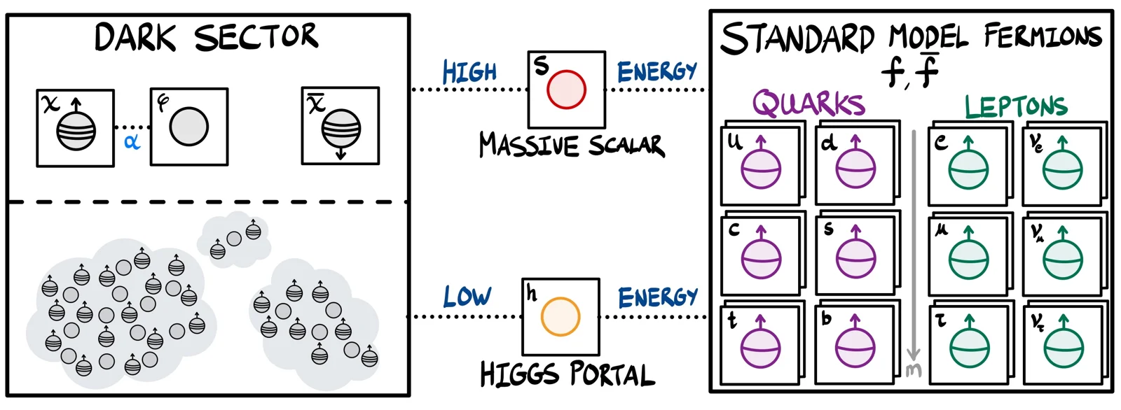
The sketch above shows how this dark sector connects to us. At very high temperatures, a heavy scalar $S$ couples to both the dark fermions and ordinary fermions, which keeps the two sectors at the same temperature. As the Universe cools, this contact switches off and the dark sector is left on its own. For it to be on its own before the dark fermions freeze out, $S$ has to be heavy. For order-one couplings this needs $m_S \gtrsim 10^7\ {\rm GeV}\,(m_\chi/1\ {\rm GeV})^{1/2}$. At low energies the only remaining link is a very weak mixing between $\varphi$ and the Higgs. I’ll come back to that at the end.

One more ingredient is that the dark matter is asymmetric. There are slightly more fermions than antifermions, just as there is slightly more matter than antimatter in our sector. When the pairs annihilate, a leftover population of fermions remains, with no antiparticles left to destroy whatever they build.

Three steps in the early Universe#

The figure below shows a schematic of one history from the paper, drawn to match our numerical solutions, with the energy in each component plotted against the temperature of ordinary radiation. The Universe cools from left to right. In this example $m_\chi = 10$ GeV, $\alpha = 0.1$ and $m_\varphi = 1$ meV.

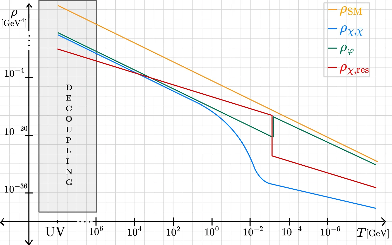
Step one, freeze-out. Once the temperature falls below the fermion mass, fermion–antifermion pairs annihilate into pairs of scalars, $\chi\bar\chi \to \varphi\varphi$. The blue curve drops as the symmetric part of the dark matter disappears. Since the sector is secluded, every bit of that energy goes into $\varphi$. The asymmetric leftovers, in red, carry on.

Step two, dark hydrogen. The leftover fermions first pair up. When the scalar is light enough, $m_\varphi \ll \alpha m_\chi$, the force between two fermions is effectively Coulombic, so each pair is a dark hydrogen atom. We worked out the dark hydrogen atom in Part I, $E_{\rm bind} = \tfrac12\alpha^2\mu$, and for two equal masses the reduced mass is $\mu = m_\chi/2$. So the binding energy is

For our example that is $25$ MeV, a quarter of a percent of the fermion mass. Pairs start to form once the Universe is cool enough that collisions stop breaking them apart, which we take to be around $T_{\rm form} \simeq BE(2)/10$, or about $2.5$ MeV here. Pairing alone releases very little energy.

Step three, building big. Pairs then merge with pairs, and composites with composites, $X_N + X_N \to X_{2N} + \varphi$, until merging becomes too slow to keep up with the expansion of the Universe. This is where the action is. In the figure, the red curve plunges by many orders of magnitude and the green curve jumps up to meet it. In one step, most of the dark matter’s mass has turned into scalar radiation.

How much mass does a fermion lose?#

That plunge in the red curve is so large that it is worth seeing where it comes from. A big composite is a ball of fermions much larger than the range $1/m_\varphi$ of the force. Inside it, the scalar field takes a large value $\varphi \approx m_\chi/g$ that cancels nearly all of the fermion mass, so the fermions inside move almost like massless particles. The question is then what it costs to hold them together, and the answer comes from balancing two energies.

The first is the energy of the fermions themselves. Pack $n$ of them per unit volume and the Pauli principle forces them to fill momentum states up to the Fermi momentum $p_F = (3\pi^2 n)^{1/3}$. For nearly massless fermions the average energy per fermion is $\tfrac34 p_F$.

The second is the energy stored in the scalar field. Holding the field at $\varphi \approx m_\chi/g$ costs a potential energy density $\tfrac12 m_\varphi^2\varphi^2 \approx m_\varphi^2 m_\chi^2/(2g^2)$, which shared among $n$ fermions is $m_\varphi^2 m_\chi^2/(2g^2 n)$ each.

The energy per fermion is therefore

Packing the fermions closer costs Fermi energy, and spreading them out costs field energy, so the nugget settles at the density in between. Minimizing over $n$ gives $\tfrac14(3\pi^2)^{1/3} n^{-2/3} = m_\varphi^2 m_\chi^2/(2g^2 n^2)$, and at that density the energy per fermion works out to be exactly the Fermi momentum,

This simple balance reproduces the effective mass of a fermion inside a saturated composite that we use in the paper, which we take from earlier work ². The density it picks does not depend on how many fermions there are, which is the saturation we talked about in Part I.

Now put in numbers. For $m_\chi = 10$ GeV and $\alpha = 0.1$, a scalar of $1$ eV gives $\bar m_\chi \approx 0.3$ MeV, and a scalar of $1$ meV gives $\bar m_\chi \approx 8$ keV. With the 1 meV scalar, a 10 GeV fermion that joins a composite ends up behaving like something about a million times lighter. Each fermion sheds $m_\chi - \bar m_\chi$, nearly its whole mass, and in a secluded sector all of that becomes $\varphi$.

Why a lighter glue leaves more behind#

The formula also contains a result that runs against intuition. Because $\bar m_\chi \propto m_\varphi^{1/2}$, a lighter scalar means more energy is radiated. You might expect the mass of the glue to matter little, but think about what we need at the end. The dark matter has to come out at today’s observed density. If the fermions are going to lose a larger fraction of their mass, there must have been more of them to begin with, and that larger initial population means more $\varphi$ after assembly.

We can turn this into a rough estimate of how much $\varphi$ is around when it matters. This is my own back-of-the-envelope version, since in the paper we solve the Boltzmann equations numerically. Right after assembly, the energy in $\varphi$ is about $m_\chi/\bar m_\chi$ times the energy in the composites. From then on, $\varphi$ is radiation and its energy density falls as $a^{-4}$ with the scale factor $a$, while the composites are matter and fall as $a^{-3}$. Their ratio therefore falls in proportion to the temperature, by a factor $T_{\rm eq}/T_{\rm form}$ by the time of matter–radiation equality, $T_{\rm eq} \simeq 0.8$ eV. At equality the composites match the ordinary radiation, so

Using $T_{\rm form} \simeq m_\chi\alpha^2/40$ and the formula for $\bar m_\chi$, this scales as

For our example it comes out at about $0.4$ for $m_\varphi = 1$ meV and $0.01$ for $m_\varphi = 1$ eV. The estimate ignores some bookkeeping that the full calculation includes, but it gets the trends right. There is more leftover $\varphi$ for a lighter scalar, and less for a heavier fermion or a stronger coupling, because those make the composites form earlier and give the $\varphi$ radiation longer to dilute.

Reading the record in the CMB#

What happens to all that $\varphi$ depends on its mass.

If $\varphi$ is lighter than about an eV, it is still moving close to the speed of light at matter–radiation equality, and it behaves as extra radiation. Cosmologists measure extra radiation through the effective number of neutrino species $N_{\rm eff}$, which counts it in units of one neutrino species. Planck measures $N_{\rm eff}$ to within a few tenths ³, and CMB-S4 is designed to get down to a few hundredths ⁴. In the full calculation we find that Planck already rules out part of the parameter space for scalar masses between about 100 μeV and 1 eV, and that CMB-S4 would reach further.

The biggest uncertainty is exactly when the composites form. Gresham, Lou and Zurek found that composites breaking apart during assembly push the effective formation temperature somewhere between $BE/10$ and $BE/30$ ⁵, so we show our results for both ends of that range.

If $\varphi$ is heavier than about an eV, it slows down before equality and behaves like matter instead. It then becomes a small extra component of the dark matter, sitting alongside the composites. Requiring that the two together do not add up to more dark matter than we observe rules out more of the parameter space. What a $\varphi$ component of dark matter would do after that is a question we left for future work.

Either way, the remnant field is a signal you could see without ever detecting a composite.

And catching the composites themselves#

The weak mixing between $\varphi$ and the Higgs is what connects all of this to experiments on Earth. It has to be tiny. The Higgs can decay into pairs of scalars, and keeping that from overproducing $\varphi$ requires the portal coupling to satisfy $\lambda_{h\varphi} \lesssim 4\times10^{-8}$ ⁶. With a coupling that small, a single $\varphi$ scattering off a nucleon has a cross section of at most about $10^{-53}$ cm², far below the reach of any current experiment.

This is where Part I’s main lesson comes back. A nucleus does not have to hit one $\varphi$. It can fly into a composite, where the scalar field is enormous, $\varphi \sim m_\chi/g$, and feel a potential produced by the whole composite at once. The strength of that potential for a nucleon is

and Acevedo, Bramante and Goodman showed that nuclei crossing such a potential recoil in a way xenon experiments can detect for couplings as small as $g_N \sim 10^{-17}$ ⁷. The scalar couples so weakly that you would never see it one particle at a time, but the composite collects its effect and makes it visible. The same mixing is limited by stellar cooling ⁸, by fifth-force tests and by cosmology, and the paper maps out where these limits leave room.

What I take away from this#

The picture I like is that the same binding field gives two separate ways to find this kind of dark matter. The composites might turn up in an underground detector. The energy released in building them might show up in the CMB. Even if the dark sector stopped talking to us long before the composites formed, the act of building them would have left radiation behind, and that is something we can measure.

There is plenty left to do. We assumed the two sectors started at the same temperature, which need not be true. And it would be interesting to look at cases where the composites form very late, after matter–radiation equality, because a burst of $\varphi$ released that late could leave its own distinct imprint on the CMB.